Types of Data

• Types of data include:
  • Non-numerical/qualitative/categorical
    • When a variable/observation can only belong to a distinct category
    • Includes nominal & ordinal

Nominal	Unordered & mutually exclusive categories. Not possible to rank Examples – alive/dead, blood group
Ordinal	Ordered  & mutually exclusive categories. Can be ranked. Difference or ‘gap’ between values can be ill-defined, Examples – mild/moderate/severe

• Numerical/quantitative
  • When a variable/observation takes a numerical value
  • Can be continuous (infinitely dividable) or discrete (whole numbers)
  • Continuous data includes interval & ratio

Interval	Continuous, no reference. No ‘none’ or ‘true zero’ available. Difference or ‘gap’ between observations is equal at all points on the scale. Examples – temperature
Ratio	Continuous, with reference. There is a reference  or ‘zero’ Difference or ‘gap’ between observations is equal at all points on the scale. Examples – pain scores

• Data can be converted to different types for analysis BUT this results in information loss and statistical power loss

Summarising Data

• Statistical methods used for summarising data depend on the type of data your dealing with 

Measure of typical value
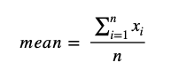
Mean (x̄ is the sample mean, μ is the population mean) – also known as the arithmetic mean – add up all numbers & divide by sample size
Geometric mean – used for right/positively skewed data – to do this, you need to take the log of each value, then calculate the mean, then back transform
Weighted mean – if certain variables are of particular interest, then a weighting can be added to those values
Median – middle value (or average of 2 middle values)
Mode – most common value

Measures of variance/spread
Range – difference between minimum and maximum value
Median – middle value (or average of 2 middle values)
Interquartile range – 25th to 75th centile
Standard deviation (σ) – square root of variance
Variance = The average of the squared differences from the mean. (First calculate the mean of a dataset. Then the difference between a data point and the mean. Square this difference, ie “squared differences”. The average of squared differences is the mean)

Frequency tables
Need statistical tests to interpret

Graphs
Visually illustrate frequency or proportion relative frequency (i.e. %)
Categorical or discrete – tend to use bar, pie chart
Continuous – tend to use histogram, dot plot, stem & leaf plot, box plot
If 2 continuous variables – can use scatter diagram
chart

Example:

Data: 13, 17, 21, 26, 27, 32

Stem and Leaf Plot:

13,   17,   21,   26,   27,   32
Stem	Leaf
1	3     7
2	1     6     7
3	2

• Numerical/quantitative data
  • Summary statistics chosen depends on whether the data has a normal or non-normal distribution
  • Numerical/quantitative data can be described by using measures of the typical value and also measures of spread…

Mean equation:

Standard deviation equation (for a sample):

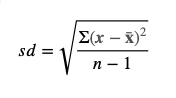
Where x is data value; x̄ is sample mean; n is sample size; Σ (sigma) means the “sum of”. Note the denominator for standard deviation of a population is “n” and not “n-1”. The -1 factor is used to account for a degree of error when SD is calculated for a sample.