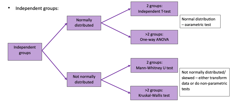
• Decision on which statistical test to use for hypothesis testing depends on:
  • Type of data (continuous or categorical)
  • Whether the groups are independent or paired
  • Whether the data is normally distributed or not
  • Number of groups

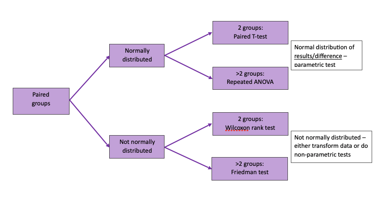
CONTINUOUS OUTCOMES

• Paired groups:
  • Repeated data on the same groups of patients e.g. before & after intervention

CATEGORICAL OUTCOMES

• E.g. percentages or proportions
• Will usually be shown in a table

CORRELATION AND REGRESSION

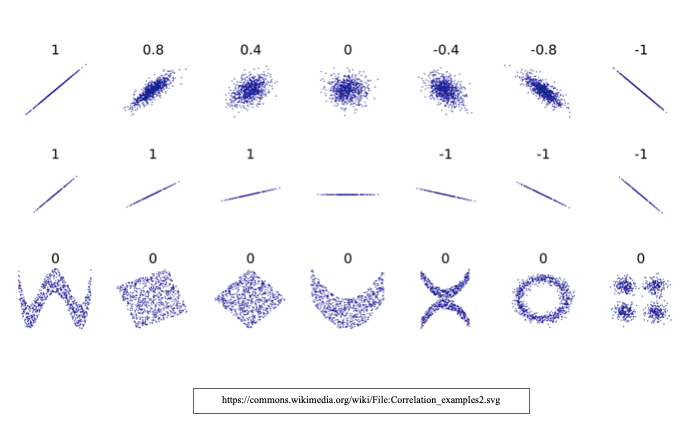
• Correlation – concerned with strength (how close the points are to the straight line) & direction of association between variables 
• Correlation coefficient – a quantitative measure, ranging from -1 to +1, of which the extent to which points in a scatter diagram conform to a straight line
• Regression – demonstrates gradient (to what degree output [y] will change when input [x] changes) & direction of an association between variables
• Regression coefficient – the parameters (i.e. the slope and intercept in simple regression) that describe a regression equation
• Use scatter plots to aid examination between relationship between variables

Correlation

• Correlation analysis is concerned with strength (how close the points are to the straight line) & direction of association between variables
• Does not matter which variable is on the x & y axis as it does NOT infer causation
• Calculates correlation coefficient, ranging from 1  0  +1 which indicates strength and direction of association
  • Negative – Y goes down as X goes up
  • No association (0) – no relationship
  • Positive – Y goes up as X goes up

• Types of correlation tests:
  • Pearson’s correlation
    • Use only If the data is parametric (normally distributed)
    • Sensitive to extreme outliers
  • Spearman’s correlation
    • If the data is non-parametric (not normally distributed/skewed)

• Disadvantages
  • Does not indicate magnitude of relationship
  • Can only compare 2 variables
  • You cannot calculate the correlation coefficient in these circumstances:
    • When the relationship is not linear
    • In the presence of outliers

Regression

Types:

• Continuous data with linear relationship —> linear regression
• Multiple variables –> multivariate regression
• Binary outcome —> logistic regression
• Survival —> cox regression

• Linear regression
  • To define the relationship between variables & allows prediction of information
  • Establishes magnitude/gradient& direction of relationship = if X (input) ↑ by 1, predicts how that will affect Y (output)
  • Linear regression equation
    • y = mx + c
    • y is the output (outcome)
    • x is in the input (dependent variable)
    • c is the y axis intercept
    • m = slope of the straight line

In the graph above – the red dots are observations. The green lines represent random variability/deviations and the blue line represents the actual true relationship between the outcome (y) and the dependent variable (x). For example if x was number of fruits/veg. eaten per day in the third trimester and y was the birth weight in pounds of the baby. This graph would show a linear relationship between the two. The more fruits/veg per day, the heavier the baby. (completely made up example!!)

• Fit statistics (R²)
  • Tells us strength of relationship from regression model
  • For a 2 variable linear regression – R² is the same as the pearson’s correlation squared
  • Ranges from 0 –> 1 (does not give direction)

• Multivariate regression
  • Allows multiple predictor/X variables
  • Adjusts for/controls for or removes effects of confounding factors
  • y = m₁x₁ + m₂x₂ + m₃x₃ + m₄x₄ ….. + c

• Logistic regression
  • Outcome is binary (2 categories – yes/no)  
  • Probability of outcome = proportion of yes (changes binary data to number – 0.2 or 20%)
  • Proportion = P = ranges from 0–>1
  • Odds = p/(1-p) = ranges from 0 to infinity
  • Log odds = ranges from -infinitiy to +infinity
  • Allows us to do modelling/linear regression on a binary outcome
  • The anti-log/exponent of the log odds is the odds ratio
    • Explains how the probability of Y changes for a 1 unit increased in X
    • As this is a RATIO – no effect =1 OR, <1=decreased probability with increasing X, OR>1=increased probability with increasing X
    • E.g. cancer occurrence = exposure to asbestos (weeks)
    • OR=1.2 –> 20% more likely for cancer to occur for every week exposed to asbestos